Speech recognition is not just a model problem. When you use an STT model like Whisper, the model handles the core inference that converts speech to text — but the condition of the audio going into the model has a large impact on results. Even for the same utterance, if the microphone is far away, keyboard noise bleeds in, an air conditioner's low-frequency hum underlies everything, or the recording level is too low, the model receives a much harder input.
This is the first post in the STT series, covering how to think about audio noise and what order to apply preprocessing steps. The goal is to help beginners understand the overall shape of a pipeline. Rather than walking through specific library APIs, I'll explain what each step does and why.
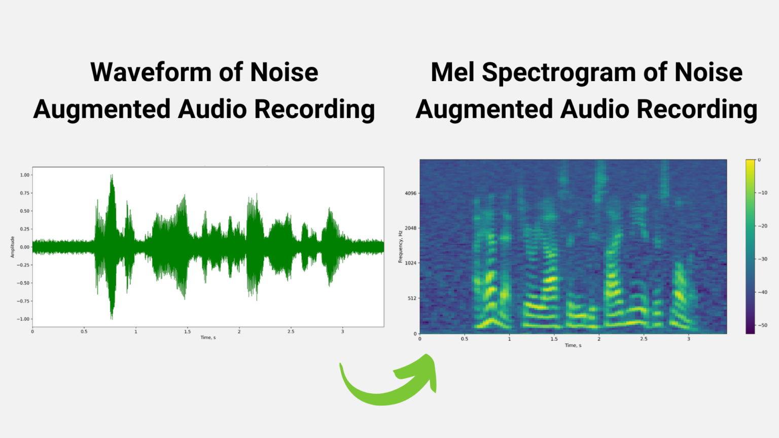
Automatic speech recognition can be understood as a pipeline that converts raw audio input into features, passes them through a model, and outputs text. Source: NVIDIA Technical Blog
Audio preprocessing is about cleaning up the input before the model
An STT model does not directly convert raw sound into sentences. Typically, input audio is normalized to a fixed sampling rate and channel format, segmented into short time windows, and then transformed into features that represent frequency content. The Whisper paper describes an architecture that converts 30-second audio segments into log-Mel spectrograms and feeds them into a Transformer encoder-decoder model.
The key point here is that what the model "hears" is not sound as humans perceive it — it's a signal that has been digitized according to a fixed set of rules. Poor recording quality leaves noise in those digitized features, and that noise interferes with the model's ability to distinguish phonemes and words.
The goal of preprocessing is not simply to make audio sound better. It's to clean up the input signal so that the STT model can more reliably extract speech information.
Noise is not a single thing
When people say "audio noise," they usually picture "loud background sound," but in practice there are several distinct types. The type determines the appropriate treatment.
- Stationary noise: Continuous, steady-state sounds like air conditioners, fans, PC cooling systems, or refrigerators.
- Transient noise: Short, impulsive sounds like keystrokes, mouse clicks, door slams, or cup impacts.
- Background speech: Other people talking nearby. This is often harder to deal with than music.
- Reverberation: The effect of a voice reflecting off walls and arriving delayed, mixing with the direct signal.
- Clipping: Distortion that occurs when the input level is too high and the waveform is truncated at its peaks and troughs.
- Low-frequency rumble: Low-frequency noise concentrated from desk vibration, microphone handling, or wind.
Stationary noise responds reasonably well to filtering or noise-profile-based removal. Transient noise and background speech are much harder. Background speech in particular is difficult to separate with simple filters because, from the STT model's perspective, it is another speech signal — not noise.
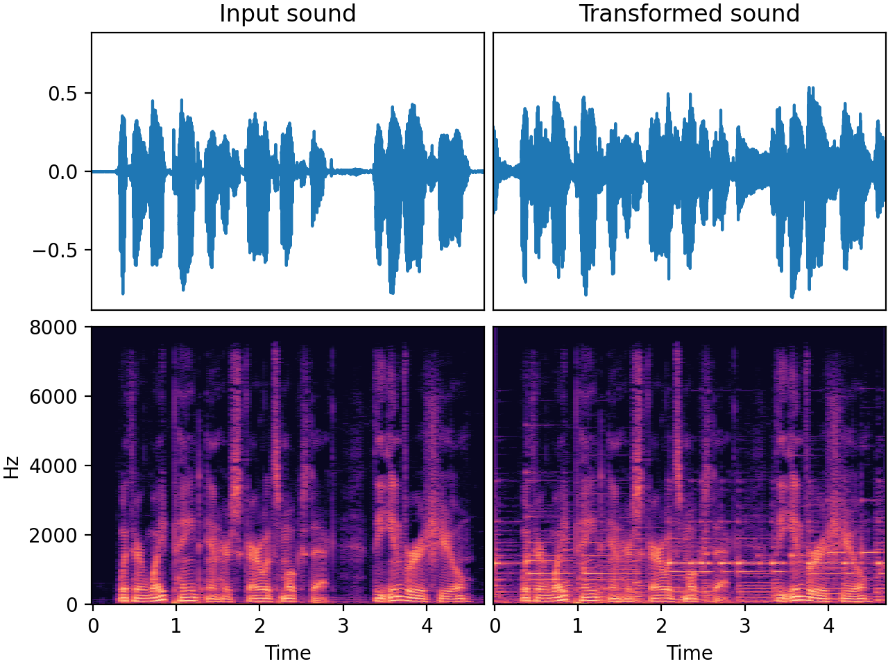
When background noise is mixed in, energy remains even during silence segments in the waveform. Source: audiomentations documentation
The first thing to look at is the waveform
Beginners often jump straight to models or complex algorithms for audio preprocessing. But the first step is to look at the waveform. A waveform shows how the amplitude of sound changes over time.
What you can see in a waveform is simple but important:
- Whether the speech was recorded at too low a level.
- Whether the input level was too high and clipping occurred.
- How much noise is present during non-speech segments.
- Whether there are sudden clicks or impact sounds.
- Whether silence and speech segments are roughly distinguishable.
If the waveform is already severely clipped, recovery in later steps is difficult. Clipping is not just a volume problem — it means part of the original signal has been lost entirely. This is why it's safer to record with a bit of headroom rather than driving the input level too hard.
A spectrogram is a frequency map of sound over time
Looking at the waveform alone makes it hard to distinguish pitch characteristics and noise type. That's where spectrograms come in. A spectrogram shows both the time axis and frequency axis together, using color brightness to represent energy level.
The human voice spans a wide frequency range, but most of the information relevant to speech is concentrated in certain bands. Conversely, wind noise and desk vibration tend to concentrate in low frequencies, while electrical hiss noise often appears as a thin layer across high frequencies.
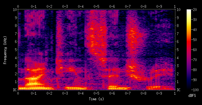
A spectrogram shows how frequency content changes over time, represented by color. Source: Wikimedia Commons
From a spectrogram, you can make the following judgments:
- If noise is concentrated only in low frequencies, a high-pass filter may help.
- If a particular frequency band shows up persistently as a bright line, consider hum removal or a notch filter.
- If the full frequency range is bright even during non-speech segments, stationary noise is significant.
- If speech and background music overlap, the problem becomes source separation rather than simple noise reduction.
Models like Whisper also convert audio internally into log-Mel spectrogram form before processing. The Whisper implementation processes audio at 16 kHz and constructs a Mel spectrogram as the model input. Understanding spectrograms gives you a concrete picture of what the STT model actually sees.
Keep the baseline pipeline simple
Starting immediately with a complex speech enhancement model is not a good approach. The more preprocessing steps you add, the greater the risk of degrading the speech itself. A baseline pipeline should be simple.
Keep the pipeline simple: input normalization, light filtering, loudness normalization, VAD, then STT input.
The flow I use as a starting point is:
- Read the input file.
- Convert to mono.
- Resample to the sampling rate expected by the STT model.
- Lightly attenuate very low-frequency rumble.
- Normalize loudness to an appropriate level.
- Use VAD to separate speech and non-speech segments.
- Apply noise reduction only when needed.
- Segment long audio into chunks that fit the model's input window.
- Feed into the STT model.
The core idea here is not "aggressively remove everything" — it's "organize the signal into the form the model needs."
Resampling and mono conversion are about matching input specs
The sampling rate is the number of times per second that sound is measured. A 48 kHz audio signal is sampled 48,000 times per second; a 16 kHz signal is sampled 16,000 times per second. STT models and preprocessing libraries often operate at a specific expected sampling rate.
Whisper processes audio at 16 kHz. So rather than feeding in a 44.1 kHz or 48 kHz recording directly, the standard approach is to resample to 16 kHz first. Functions like librosa's resample handle converting an audio time series to a different sampling rate.
Stereo audio has separate left and right channels. For STT purposes, collapsing to mono is usually sufficient. Meeting recordings where each channel contains a separate speaker may require individual handling, but for typical microphone input, mono conversion keeps the pipeline simple.
Filtering attenuates specific frequency bands
Filters are how you clean up audio based on frequency content. They're not a magic step that removes all noise, but they're highly effective in specific situations.
- High-pass filter: Attenuates very low frequencies. Used to reduce rumble from microphone handling, wind, and desk vibration.
- Low-pass filter: Attenuates very high frequencies. Used sparingly when high-frequency hiss is severe.
- Band-pass filter: Retains only a specific frequency range. Used when you want to focus on the speech band.
- Notch filter: Narrows and attenuates a single specific frequency. Used to remove narrow-band noise like power-line hum.
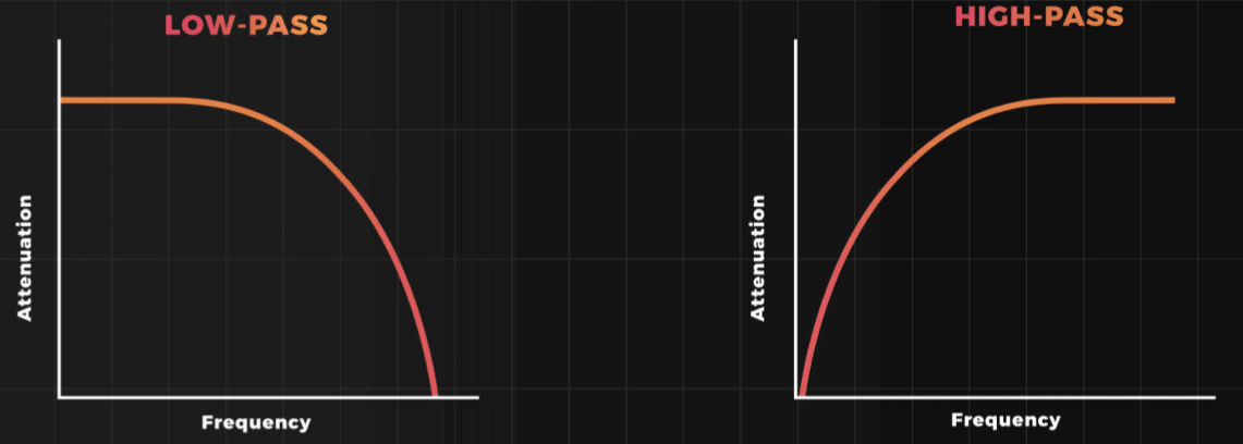
Filters clean up a signal by attenuating or passing specific frequency bands. Source: Unison Audio
Applying filters too aggressively will also remove parts of the speech. In particular, consonant information is tied to high-frequency components, so an overly aggressive low-pass filter can impair phoneme discrimination. In STT preprocessing, what matters more than making the audio sound smooth to human ears is whether the information the model needs to distinguish words is still present.
Loudness normalization is about matching levels, not just making things louder
Normalization adjusts overall loudness to a consistent reference level. Beginners often think of normalization as "turning up the volume," but the real goal is to stabilize the input level.
If speech is recorded too quietly, the gap between noise and speech narrows. If it's too loud, clipping can occur or the model's input features can be distorted. That's why normalization is an important step independent of noise reduction.
This is where the concept of SNR comes in. SNR — signal-to-noise ratio — represents the relative level of the speech signal versus background noise. A higher SNR is favorable for STT. Simply amplifying the entire signal raises both speech and noise equally, so it does not actually improve the SNR.
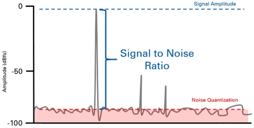
SNR is the fundamental concept for understanding the relative difference between speech signal and background noise. Source: Chris's Sound Lab
Normalization is about matching input scale; noise reduction is about changing the relationship between signal and noise. These are distinct goals.
VAD is the step that finds where speech occurs
VAD stands for voice activity detection. It identifies which segments of the input audio contain speech and which do not. VAD is critically important in STT preprocessing.
Removing non-speech segments reduces the amount of unnecessary noise the model has to process. For long recordings, it also provides a basis for segmenting audio by utterance. In models like Whisper that process input in fixed-length windows, the VAD and chunking strategy has a direct impact on both output quality and processing speed.
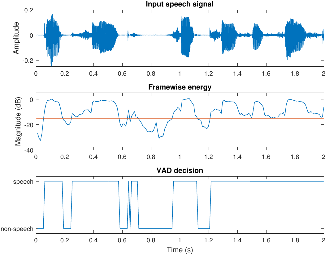
VAD is used to classify short frames as either speech or non-speech. Source: Introduction to Speech Processing
py-webrtcvad is the standard Python package for using WebRTC VAD. WebRTC VAD makes speech/non-speech decisions on short frames — typically 10 ms, 20 ms, or 30 ms — and exposes an aggressiveness parameter that controls how strictly it filters out non-speech.
Setting VAD too aggressively can clip soft speech or cut off sentence endings. Setting it too loosely leaves too many noise segments. In practice, VAD is typically applied with a small amount of padding around detected speech regions — sometimes called hangover — to avoid these boundary artifacts.
Apply noise reduction last, and conservatively
Noise reduction is an attractive step, but it doesn't always improve STT results. If a noise reduction algorithm also attenuates parts of the speech signal, it can make things harder for the model rather than easier.
The classic approach is spectral gating: estimate a noise profile from a non-speech segment, then subtract that pattern from the spectrum of the full signal. The Audacity noise reduction workflow describes this profile-based approach, with controls for reduction amount, sensitivity, and frequency smoothing.
Deep learning-based approaches also exist. RNNoise is a well-known example that uses a recurrent neural network for real-time noise suppression. These methods can be effective against stationary noise and general background noise, but they can also introduce artifacts — changing the texture of speech or softening consonants.
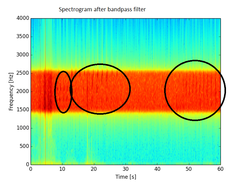
Noise reduction can be understood as attenuating noise components in the spectrum. Source: DSP Stack Exchange
For STT purposes, it's safer to apply noise reduction lightly and compare recognition results before and after, rather than going in aggressively. Audio that sounds better to human ears is not always audio that an STT model reads more accurately.
Chunking splits long audio into units the model can process
Long files often can't be fed in all at once. Whisper is designed around 30-second audio windows, so processing a long meeting or broadcast recording requires chunking it into appropriately sized segments.
The critical concern in chunking is avoiding cuts in the middle of sentences. Cutting mid-word or mid-sentence loses context on both sides and can cause recognition errors. The standard approach is to use VAD to identify speech boundaries and, for utterances that are too long, split them with overlapping regions.
This overlap is called — unsurprisingly — overlap. For example, even when cutting into 30-second segments, overlapping the boundaries by about 1 second on each side makes it easier to recover words that fall at an edge. The tradeoff is that you need to deduplicate overlapping output when merging results.
Common mistakes in STT preprocessing
Beginners tend to make the same mistakes repeatedly:
- Applying noise reduction too aggressively.
- Mixing multiple formats without resampling.
- Not distinguishing between stereo and mono.
- Leaving large amounts of silence segments in the input.
- Trying to fix clipping with normalization.
- Ignoring word-boundary artifacts at chunk edges.
- Evaluating by listening and judging it "sounds better," without comparing actual STT output.
Preprocessing decisions should always be validated against recognition results. For the same file, compare the original, a lightly preprocessed version, and an aggressively noise-reduced version side by side — that's how you find out what actually helps.
Minimum preprocessing as a practical starting point
If you're building an STT pipeline for the first time, the following is a realistic baseline:
- Convert input to mono.
- Resample to 16 kHz.
- Check for clipping.
- Lightly attenuate only the lowest-frequency rumble.
- Normalize loudness to an appropriate level.
- Use VAD to locate speech segments.
- Segment long audio at utterance boundaries.
- Apply noise reduction only to files that need it, and lightly.
- Compare STT results before and after preprocessing.
This setup is simple but solid. Instead of applying the same heavy corrections uniformly to all audio, it focuses on organizing the signal into a form the model can read reliably.
Thinking About It in Code
The exact implementation depends on which libraries you use, but the overall flow is roughly the same.
waveform, sr = load_audio(path)
waveform = to_mono(waveform)
waveform = resample(waveform, orig_sr=sr, target_sr=16000)

waveform = high_pass_filter(waveform, cutoff_hz=80)
waveform = normalize_level(waveform)

segments = detect_voice_segments(waveform, sr=16000)
chunks = make_chunks(waveform, segments, max_seconds=30, overlap_seconds=1)

texts = []
for chunk in chunks:
    clean_chunk = optional_noise_reduction(chunk)
    text = stt_model.transcribe(clean_chunk)
    texts.append(text)

result = merge_texts(texts)
This is less finished code and more a sketch of the reasoning order. What matters is understanding why each step exists. Resampling matches the expected input format. The filter knocks down clear frequency artifacts. VAD finds the speech regions. Chunking fits the audio into the model's input window.
Good Preprocessing for STT Is Conservative
Audio preprocessing is not a case where more is better. Good preprocessing does only what is necessary. In STT especially, the goal is not to make audio sound polished the way you might for music — it is to preserve as much of the identifying information in the speech signal as possible while making the model less sensitive to noise it does not need to care about.
To summarize: the first principle is to match the expected input spec. The second is to remove segments where no one is speaking. The third is to reduce only unambiguous noise, and to do so carefully. The fourth is to always compare STT output before and after preprocessing.
Following these four principles will give you much more stable audio input quality across tasks like Whisper inference, TTS/STT experiments on OmniVoice, real-time voice agents, and automated meeting transcription.