1편에서 원리를 다루고 2편에서 적용 방식과 모델별 특징을 살펴봤다면, 3편에서는 직접 실험해볼 차례다. Speculative decoding은 논문에서 끝나는 기법이 아니다. Hugging Face Transformers, vLLM, TensorRT-LLM 같은 추론 스택에 이미 실험 가능한 형태로 통합되어 있으며, 코드 생성, RAG, 챗봇, 배치 추론에서 각각 다른 양상을 보인다.
먼저 버려야 할 기대가 하나 있다. 옵션 하나를 켜면 모든 요청이 빨라지는 방식으로 동작하지 않는다. 같은 모델이라도 프롬프트 종류, 출력 길이, 샘플링 설정, batch size, draft 방식에 따라 결과가 달라진다. 실무에서는 "speculative decoding을 쓴다"보다 "어떤 요청군에서 accept rate가 높고, GPU 메모리와 지연 시간이 어느 정도로 움직이는가"가 더 중요하다.
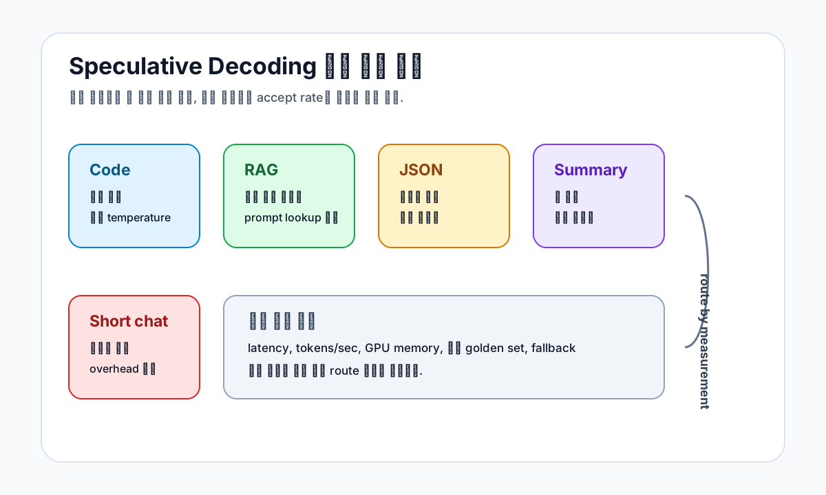
그림 1. speculative decoding은 요청 유형별로 적용 후보가 달라진다.
실험 전에 잡아야 하는 기준선
Speculative decoding을 붙이기 전에 기본 서빙 성능을 먼저 측정해야 한다. 이 순서를 건너뛰면 빨라졌는지 느려졌는지 판단할 기준이 사라진다. 특히 초보자에게 자주 나타나는 착시는 첫 토큰 지연 시간과 전체 토큰 처리량을 섞어서 보는 데서 비롯된다.
서빙 성능은 최소한 아래 항목으로 나눠서 측정한다.
| 지표 | 의미 | 왜 봐야 하는가 |
|---|---|---|
| TTFT | Time To First Token | 사용자가 체감하는 첫 응답 속도 |
| TPOT | Time Per Output Token | 긴 답변 생성 중 토큰당 지연 |
| End-to-end latency | 요청 전체 완료 시간 | 실제 API 응답 시간 |
| Output tokens/sec | 초당 생성 토큰 수 | 처리량 비교 |
| GPU memory | 모델, KV cache, draft 비용 | 동시성 한계 |
| Accept rate | draft token 중 target이 받아들인 비율 | speculative decoding의 효율 |
Accept rate는 반드시 확인해야 한다. draft가 토큰 5개를 제안했는데 target이 매번 1개만 받아들인다면, 작은 모델을 추가로 실행한 비용이 그대로 손실이 된다. 반대로 코드처럼 반복 패턴이 많거나, RAG 답변처럼 컨텍스트를 거의 그대로 옮기는 출력에서는 여러 토큰이 연속으로 accept될 가능성이 높아진다.
실무에서 내가 잡는 최소 실험 단위는 요청 30개다. 엄밀한 벤치마크라기보다는 "이 설정이 말이 되는가"를 확인하는 스모크 테스트에 가깝다. 요청은 짧은 질의, 긴 질의, 코드 생성, 요약, RAG 답변처럼 유형별로 분리한다. 섞어서 평균을 내면 어떤 요청에서 이득이 있었고 어떤 요청에서 손해를 봤는지 바로 묻혀버린다.
baseline/
  chat_short.jsonl
  chat_long.jsonl
  code_completion.jsonl
  rag_answer.jsonl

speculative/
  same_prompts_same_sampling.jsonl
비교할 때는 프롬프트와 sampling 설정을 고정한다. temperature, top_p, max_tokens가 달라지면 speculative decoding의 효과가 아니라 생성 조건의 차이를 보는 셈이 된다.
사례 1: Hugging Face Transformers에서 assistant model로 감 잡기
가장 쉽게 시작하는 방법은 Transformers assisted generation이다. 큰 모델을 target으로 두고, 작은 모델을 assistant로 붙인다. 여기서 assistant model은 draft model 역할을 한다.
초보자에게 이 방식이 좋은 이유는 구조가 눈에 잘 보이기 때문이다. 별도 서버를 띄우지 않아도 되고, 코드 한 파일에서 target과 assistant를 함께 호출한다. 운영용 서빙 엔진을 다루기 전에 원리와 실패 양상을 확인하기 좋다.
import torch
from transformers import AutoModelForCausalLM, AutoTokenizer

TARGET = "Qwen/Qwen2.5-7B-Instruct"
ASSISTANT = "Qwen/Qwen2.5-0.5B-Instruct"

tokenizer = AutoTokenizer.from_pretrained(TARGET)

target_model = AutoModelForCausalLM.from_pretrained(
    TARGET,
    torch_dtype=torch.float16,
    device_map="auto",
)

assistant_model = AutoModelForCausalLM.from_pretrained(
    ASSISTANT,
    torch_dtype=torch.float16,
    device_map="auto",
)

messages = [
    {"role": "user", "content": "Python에서 asyncio와 thread pool의 차이를 예제로 설명해줘."}
]

prompt = tokenizer.apply_chat_template(
    messages,
    tokenize=False,
    add_generation_prompt=True,
)

inputs = tokenizer(prompt, return_tensors="pt").to(target_model.device)

with torch.no_grad():
    output = target_model.generate(
        **inputs,
        assistant_model=assistant_model,
        max_new_tokens=256,
        temperature=0.0,
    )

print(tokenizer.decode(output[0], skip_special_tokens=True))
이 예제에서 가장 먼저 맞춰야 하는 것은 tokenizer다. target과 assistant가 같은 tokenizer 계열이면 실험이 단순해진다. tokenizer가 다르면 토큰 경계가 달라지고, draft가 제안한 토큰을 target 쪽에서 그대로 검증하기 어려워진다. Transformers에는 tokenizer가 다른 assistant를 처리하는 경로도 있지만, 첫 실험에서는 같은 모델 패밀리에서 크기만 다른 조합이 낫다.
좋은 첫 조합은 아래와 같다.
| Target | Assistant | 이유 |
|---|---|---|
| 같은 패밀리 7B | 같은 패밀리 0.5B 또는 1.5B | tokenizer와 스타일이 맞을 가능성이 높다 |
| code 7B | 같은 계열 code 1B | 반복 패턴과 문법 구조를 잘 맞춘다 |
| instruct 7B | 같은 계열 instruct 소형 모델 | 채팅 포맷과 답변 톤이 덜 어긋난다 |
Assistant가 너무 작으면 draft를 빠르게 만들지만 틀릴 확률이 올라간다. 너무 크면 accept rate는 좋아져도 draft 비용이 커진다. 실험에서는 assistant latency와 accept rate를 함께 봐야 한다. accept rate만 높은 조합이 항상 가장 빠른 조합은 아니다.
같은 프롬프트로 baseline을 먼저 측정한다
아래처럼 같은 모델에서 assistant를 제거하고 한 번 더 실행한다. 이 값이 기준선이다.
with torch.no_grad():
    baseline = target_model.generate(
        **inputs,
        max_new_tokens=256,
        temperature=0.0,
    )
로컬 단일 요청에서는 큰 차이가 보이지 않을 수 있다. Python 오버헤드, GPU 메모리 배치, 모델 로딩 상태가 뒤섞이기 때문이다. 그래도 첫 단계에서는 충분하다. "동작한다", "출력이 깨지지 않는다", "assistant 조합이 말이 된다"를 확인하면 된다.
사례 2: vLLM에서 API 서버 기준으로 실험하기
운영에 가까운 실험은 vLLM speculative decoding 문서의 흐름을 따르는 편이 낫다. vLLM은 continuous batching과 KV cache 관리가 강점이라, 단일 generate 호출보다 실제 API 서버 조건을 확인하기 좋다.
명령어는 설치 버전과 지원 모델에 따라 달라진다. 구조는 아래와 같다.
vllm serve Qwen/Qwen2.5-7B-Instruct \
  --served-model-name target \
  --tensor-parallel-size 1 \
  --speculative-model Qwen/Qwen2.5-0.5B-Instruct \
  --num-speculative-tokens 4
--num-speculative-tokens는 draft가 한 번에 몇 개의 후보를 제안할지 결정한다. 처음부터 크게 잡지 않는다. 3이나 4에서 시작하는 편이 안전하다. 8 이상으로 올리면 잘 맞는 요청에서는 이득이 커질 수 있지만, 틀리는 요청에서는 버리는 토큰이 늘어난다.
API는 OpenAI 호환 엔드포인트로 호출할 수 있다.
curl http://localhost:8000/v1/chat/completions \
  -H "Content-Type: application/json" \
  -d '{
    "model": "target",
    "messages": [
      {"role": "user", "content": "FastAPI에서 dependency injection을 쓰는 이유를 예제로 설명해줘."}
    ],
    "temperature": 0,
    "max_tokens": 256
  }'
실무 실험에서는 같은 서버에서 baseline과 speculative를 번갈아 측정하기보다, 프로세스를 분리해서 측정하는 편이 깔끔하다. 한쪽은 target만 띄우고, 다른 한쪽은 speculative 옵션을 붙인다. 포트도 분리한다.
# baseline
vllm serve Qwen/Qwen2.5-7B-Instruct \
  --served-model-name baseline \
  --port 8000

# speculative
vllm serve Qwen/Qwen2.5-7B-Instruct \
  --served-model-name speculative \
  --port 8001 \
  --speculative-model Qwen/Qwen2.5-0.5B-Instruct \
  --num-speculative-tokens 4
그리고 같은 요청 파일을 두 서버에 전송한다.
import json
import time
import httpx

PROMPTS = "code_completion.jsonl"


def run(endpoint: str):
    rows = []
    with open(PROMPTS, "r", encoding="utf-8") as f:
        for line in f:
            item = json.loads(line)
            payload = {
                "model": item["model"],
                "messages": item["messages"],
                "temperature": 0,
                "max_tokens": 256,
            }
            start = time.perf_counter()
            r = httpx.post(endpoint, json=payload, timeout=120)
            elapsed = time.perf_counter() - start
            r.raise_for_status()
            data = r.json()
            usage = data.get("usage", {})
            rows.append({
                "elapsed": elapsed,
                "completion_tokens": usage.get("completion_tokens"),
                "total_tokens": usage.get("total_tokens"),
            })
    return rows

baseline = run("http://localhost:8000/v1/chat/completions")
speculative = run("http://localhost:8001/v1/chat/completions")

for name, rows in [("baseline", baseline), ("speculative", speculative)]:
    latencies = [r["elapsed"] for r in rows]
    tokens = [r["completion_tokens"] or 0 for r in rows]
    print(name)
    print("avg latency", sum(latencies) / len(latencies))
    print("tokens/sec", sum(tokens) / sum(latencies))
이 정도 스크립트만 있어도 "느낌상 빨라진 것 같다"를 벗어날 수 있다. 더 정교하게 가려면 warmup 요청, p50/p95 지연 시간, 동시 요청 수, 스트리밍 모드 TTFT를 추가한다. 처음부터 완벽한 벤치마크를 만들려고 하면 실험 자체가 멈춘다. baseline과 speculative의 차이가 충분히 큰지 먼저 확인한다.
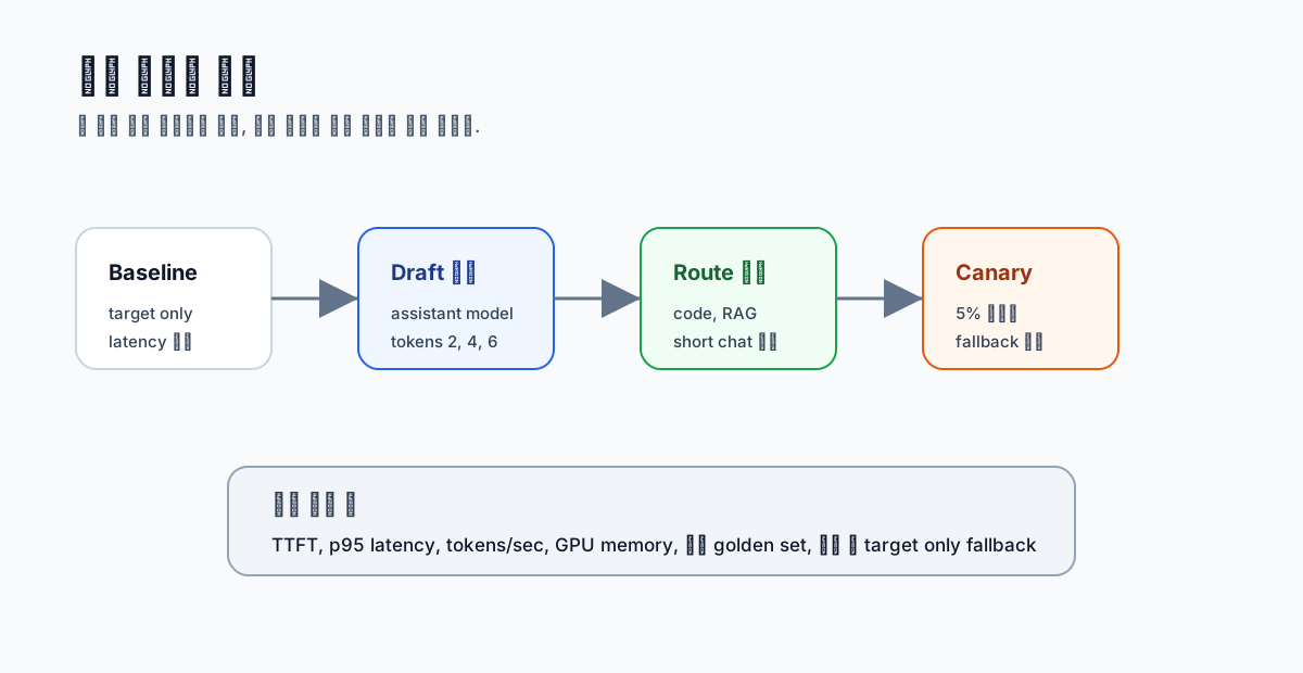
그림 2. baseline을 먼저 잡고, 작은 트래픽부터 speculative 경로로 보낸다.
Case 3: Prompt Lookup — A Good Fit for RAG and Document Q&A
There are situations where you can capture speculative-decoding-style gains without attaching a separate draft model. Prompt lookup (n-gram lookup) reuses token sequences that already appear in the prompt as candidates. As explained in Part 1, this works well when the model is reconstructing or quoting portions of the input document rather than reasoning about new knowledge.
RAG responses are the canonical example. The user's question arrives with a long retrieved document, and the answer closely mirrors the document's phrasing. In these requests, there's a high probability that the next token already appears somewhere in the prompt.
Say the input context contains this sentence:
Redis Stream은 append-only log 형태의 자료구조이며, consumer group을 사용하면 여러 소비자가 메시지를 나눠 처리할 수 있다.
If the response begins like this, a large share of the tokens overlap with n-grams from the prompt:
Redis Stream은 append-only log 형태의 자료구조다. consumer group을 사용하면...
The main advantage is that prompt lookup requires almost no additional memory — there's no second model to load. This is especially appealing when you don't have GPU headroom for a small draft model. The tradeoff is that creative generation, reasoning-heavy answers, and responses that use vocabulary not present in the prompt see limited benefit.
For beginners, I recommend two test sets:
rag_copy_heavy.jsonl    # answers that heavily quote source passages
rag_reasoning.jsonl     # answers that require synthesizing new conclusions from the document
Measure latency separately for each group. Prompt lookup will likely win on the first, while the second may show little difference — or introduce management overhead for no gain.
Case 4: Why Speculative Decoding Fits Code Generation Well
Code narrows the candidate set for the next token far more often than natural language does. Parentheses, indentation, imports, function signatures, repeated variable names, and JSON schema patterns recur constantly. This creates intervals where a small draft model can easily predict several tokens ahead.
Consider this prompt — much of the output is structurally determined before generation even begins:
FastAPI로 /healthz 엔드포인트와 /items/{item_id} GET 엔드포인트를 만들어줘.
응답 모델은 Pydantic BaseModel을 사용하고, 타입 힌트를 빠짐없이 넣어줘.
The generated code will generally follow this skeleton:
from fastapi import FastAPI
from pydantic import BaseModel

app = FastAPI()

class Item(BaseModel):
    ...

@app.get("/healthz")
def healthz():
    ...
When attaching speculative decoding to a code LLM, start with temperature 0 or a low temperature. The higher the sampling temperature, the more likely the draft and target paths diverge. Autocomplete, test code generation, and boilerplate generation are all good candidates. Conversely, algorithm problems — where intermediate reasoning can send the output in a completely different direction — will produce unstable accept rates.
For code generation, quality evaluation must accompany the speed measurement. If output speed increases but syntax errors go up, the setup is unusable in production. At a minimum, run these checks:
python -m py_compile generated.py
ruff check generated.py
pytest tests/
Relying solely on human review conflates the speed experiment with the quality experiment. Code gives you automated evaluation axes — compile, lint, test — so use them.
Case 5: Medusa and EAGLE — Look at These When the Model Is Ready
Medusa attaches multiple decoding heads on top of the target model to produce candidates for several future tokens simultaneously. Unlike the approach of calling a separate small draft model, it generates candidates within the target model itself. EAGLE predicts future hidden states at the feature level to construct the draft. Both come from the same line of thinking: generate drafts more cheaply and more accurately.
For beginners moving directly to production, these require more setup than the small draft model approach. You need a model with the heads already attached, or you need to match a supported runtime-model combination. The typical experimentation order looks like this:
- Stage 1: target-only baseline
- Stage 2: small draft model from the same model family
- Stage 3: prompt lookup or n-gram lookup
- Stage 4: Medusa or EAGLE, once the model and runtime are ready
The reason Medusa and EAGLE come last isn't that they perform worse. It's that beginners find it hard to control the experimental variables. When target, draft, tokenizer, decoding heads, and runtime support are all entangled at once, identifying the root cause of a slowdown becomes very difficult. Build intuition for accept rate and latency with a small draft model first, then move to the more advanced methods.
Roll Out by Request Type, Not All at Once
Enabling speculative decoding across all traffic simultaneously is risky. Even within the same service, requests have very different characteristics. Short greeting responses, long document summarization, code generation, RAG answers, and JSON generation all have fundamentally different decoding patterns.
Here's the routing breakdown I find works well:
| Request Type | Recommended Approach | Rationale |
|---|---|---|
| Code autocomplete | Small draft model | Low temperature, repetitive structure, long output |
| RAG citation answers | Prompt lookup | High n-gram overlap between input document and output |
| Long summarization | Small draft model or prompt lookup | Depends on how much source phrasing is reused |
| Short chatbot responses | Apply conservatively | Draft overhead can erase the gain |
| JSON / schema output | Small draft model | High structural repetition; quality is verifiable |
| Creative writing | Apply cautiously | Sampling paths diverge frequently |
Start by sending only 5% of total traffic through the speculative path. Log at least the following fields for every request:
{
  "route": "code_completion",
  "model": "target",
  "speculative": true,
  "draft_model": "assistant",
  "num_speculative_tokens": 4,
  "temperature": 0.0,
  "prompt_tokens": 812,
  "completion_tokens": 256,
  "ttft_ms": 180,
  "latency_ms": 2100,
  "tokens_per_second": 121.9,
  "accepted_tokens": 430,
  "draft_tokens": 512
}
Some runtimes don't expose accepted_tokens and draft_tokens directly. In those cases, use whatever values server metrics, debug logs, or benchmarking tools provide. If the values aren't available at all, don't contort your logs to estimate accept rate — focus on latency, throughput, and quality evaluation first.
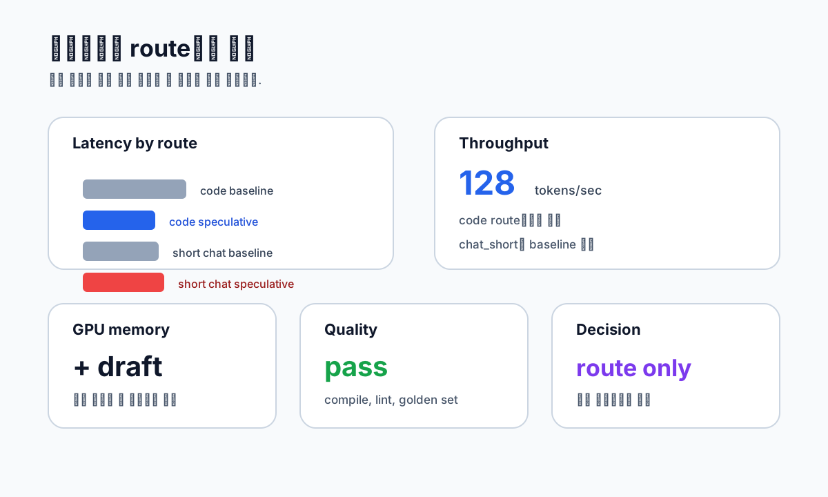
Figure 3. Looking at per-route latency, throughput, and quality together is safer than relying on a single aggregate average.
Know the Failure Patterns Before You Start
The patterns that cause speculative decoding to slow things down are fairly predictable.
First: the draft model's style doesn't match the target. Attaching a base model as the draft while using an instruct model as the target can break things at the chat format level. Even within the same model family, make sure the instruct/base alignment matches.
Second: the draft proposes too many tokens. A large num_speculative_tokens works great when the draft is right. When it's wrong, the verification step discards more tokens. In early experiments, sweep small values: 2, 4, 6.
Third: batch size and concurrency erode the gains. The draft model consumes GPU resources too. A setup where the target alone filled batches efficiently may hit scheduling issues once draft inference is added. A configuration that wins at single-request throughput doesn't necessarily win at 32 concurrent requests.
Fourth: output is too short. Responses shorter than roughly 20 tokens can't amortize the overhead of preparing and verifying drafts. Route these requests away from the speculative path.
Fifth: measuring speed without measuring quality. Speculative decoding is designed in principle to preserve the target distribution. But if the implementation, configuration, tokenizer combination, or sampling conditions are off, output quality can silently degrade. In production, maintain a golden set and continuously diff the outputs.
Experiment Order for Beginners
Don't try to evaluate vLLM, TensorRT-LLM, Medusa, and EAGLE all at once from the start. Break it into steps that can be completed in a single day.
1. Measure baseline latency with target only.
2. Prepare a fixed prompt file.
3. Attach a small assistant from the same model family.
4. Sweep num_speculative_tokens: 2, 4, 6.
5. Split request types into code, rag, and chat; record results separately.
6. Add output quality checks.
7. Promote only the winning request types to the server routing candidates.
Don't summarize results with a single average.
route=code_completion
baseline tokens/sec: 84
speculative tokens/sec: 128
latency change: -31%
quality check: pass

route=chat_short
baseline tokens/sec: 71
speculative tokens/sec: 68
latency change: +5%
quality check: pass
When you see results like these, apply speculative decoding to code generation only and exclude short chatbot responses. Rolling those two together into "12% improvement overall" obscures the operational decision.
Practical Configuration Intuition
For the small draft model approach, start with models in the 0.5B, 1B, or 1.5B range from the same family. If the target is 7B, a 0.5B or 1.5B draft is a reasonable starting point. If the target is 70B, a 7B-class draft is a candidate — but recalculate memory and parallelization costs.
Start num_speculative_tokens at 4. If the accept rate is high and outputs are long, try 6 or 8. If most responses are short, drop to 2 or remove them from the speculative path entirely.
Start with temperature 0. If your service uses temperature 0.7, benchmark that setting too. A configuration that wins under greedy decoding is not guaranteed to win under sampling.
For RAG, evaluate prompt lookup separately. If most responses heavily cite documents, you may get gains without a draft model at all. For code generation, start with a small draft model. For JSON output, include schema validation in your quality evaluation.
For heavier stacks like TensorRT-LLM — where engine builds and deployment pipelines are expensive — be even more conservative. The TensorRT-LLM speculative decoding documentation shows methods like Medusa, lookahead, and explicit draft tokens integrated tightly with runtime optimizations. In that layer, a single experiment is costly. Narrow down your model combinations and request types in vLLM or Transformers first, then move to engine-level optimization as the final step.
Production Checklist
Before putting anything into a live service, verify the following:
- A target-only baseline exists.
- The prompt file and sampling settings are fixed.
- Results are recorded separately by request type.
- p50 and p95 latency are both measured.
- TTFT and total latency are tracked separately.
- GPU memory usage and concurrency changes are monitored.
- A golden set exists for output quality evaluation.
- A decision has been made on whether to exclude short responses from the speculative path.
- A fallback to target-only exists if the draft model fails.
- Accept rate is re-measured whenever the model changes.
Re-benchmark whenever the model changes. Even swapping the target for a different instruct model of the same size can change how well it pairs with the draft. Prompt template changes also warrant re-measurement — a system prompt that strongly shifts the response style can destabilize paths the draft was previously getting right.
The next thing worth digging into is how to collect and visualize accept rate in practice. The metrics each runtime exposes vary considerably, so this is worth running a dedicated vLLM experiment to work out.