If Monte Carlo Tree Search finds strong candidates by exploring promising branches more deeply rather than expanding every possibility, Legendre approximation summarizes a complex function by keeping only its essential shape rather than memorizing it entirely. The two solve different kinds of problems, but share a clear common principle: recast computation into a tractable form and reach useful conclusions without exhaustively handling everything.
Legendre polynomials are a family of orthogonal polynomials. "Orthogonal" roughly means that two directions do not overlap. Just as the x-axis and y-axis in a vector space are independent of each other, functions in a function space can serve as a basis when they do not overlap with one another. Legendre polynomials are the canonical example of polynomials that play this role on the interval [-1, 1].
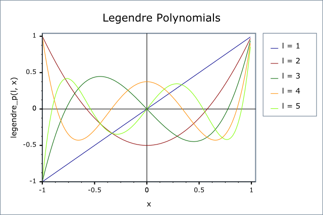
Low-degree Legendre polynomial graphs. Source: Boost C++ Libraries
The core idea I want to lay out in this post is one thing: given a complex function, expressing it as a sum of Legendre polynomials lets you summarize that function with a small number of coefficients. Those coefficients capture, level by level, information such as whether the function behaves like a constant, tilts like a line, or curves like a parabola. Legendre approximation can therefore serve as a kind of approximate inference mechanism for problems that involve continuous functions.
What Function Approximation Actually Reduces
Suppose you have a function f(x). If it is simple, you can compute it directly. The problem is that real functions are not always simple. A function may be given only as measured values, may be expensive to evaluate, or may have a known shape that is nevertheless difficult to handle in closed form.
Function approximation is the process of replacing such a function with something more tractable. Approximating sin(x) on some interval with a low-degree polynomial, or summarizing the trend in experimental data with a line or curve, are both examples of function approximation.
The key perspective here is not perfect replication. Approximation is not about reproducing the original function exactly — it is about retaining enough information for the task at hand. The goal is closer to reducing computation, suppressing noise, and extracting the structure needed for downstream inference.
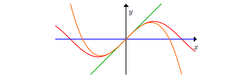
Function approximation converts the original curve into a polynomial that is easier to compute with. Source: Expii
The best analogy for a newcomer is compression. If the original function is a long audio file, Legendre approximation is like summarizing that audio with a few important frequency components. The difference from Fourier approximation is the basis: Fourier uses trigonometric functions, while Legendre uses Legendre polynomials.
What Legendre Polynomials Look Like
Legendre polynomials are usually written as P_n(x), where n is the degree. P_0(x) is degree zero, P_1(x) is degree one, P_2(x) is degree two.
The first few are:
P_0(x) = 1
P_1(x) = x
P_2(x) = (1/2)(3x^2 - 1)
P_3(x) = (1/2)(5x^3 - 3x)
P_4(x) = (1/8)(35x^4 - 30x^2 + 3)
Looking at this list, they appear to be just some unusual polynomials. But they are not arbitrary. They are constructed to be mutually orthogonal on the interval [-1, 1].
Orthogonality is expressed by the following relation:
∫[-1,1] P_m(x) P_n(x) dx = 0, m != n
Multiplying two Legendre polynomials of different degrees and integrating from -1 to 1 gives zero. In other words, information in the P_1 direction and information in the P_2 direction do not mix. This property makes it straightforward to decompose a complex function stably into separate components.
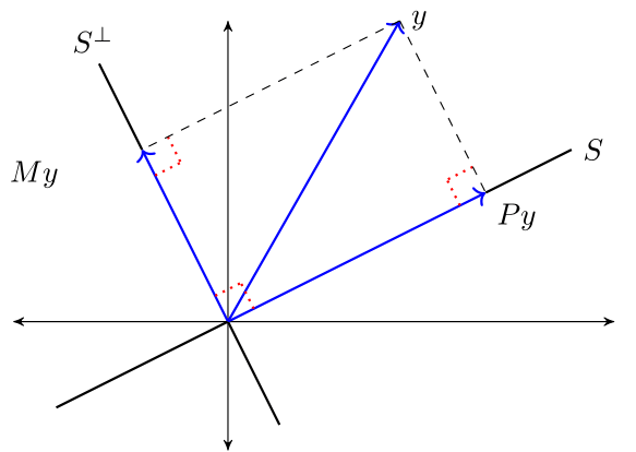
In an orthogonal basis, components can be separated and examined independently. Source: QuantEcon
The Digital Library of Mathematical Functions classifies Legendre polynomials as one family of classical orthogonal polynomials. They appear frequently in physics, numerical analysis, and approximation theory — primarily because the structure is clean and the computation is stable when you need to decompose a function over an interval into a polynomial basis.
What "Orthogonal Polynomials" Actually Means
The phrase "orthogonal polynomials" sounds intimidating at first, but the core idea is simple: a collection of polynomials whose roles do not overlap.
A 2D vector is the easiest analogy. A point (a, b) is reached by moving a along the x-axis and b along the y-axis. Because the axes are orthogonal, computing the x-component does not involve the y-component.
Functions work analogously. If a function f(x) can be written as a sum of basis functions, the contribution of each basis function can be computed independently. Legendre polynomials make the following kind of representation possible:
f(x) ≈ a_0 P_0(x) + a_1 P_1(x) + a_2 P_2(x) + ... + a_N P_N(x)
The values a_0, a_1, a_2, … are the coefficients. Each coefficient indicates how strongly the original function is expressed in the direction of the corresponding Legendre polynomial.
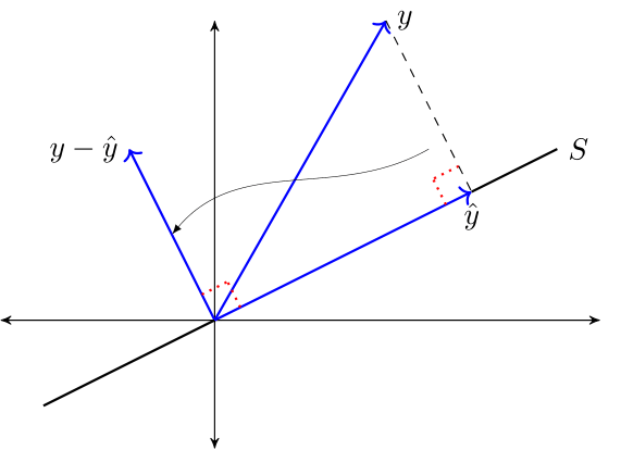
Function approximation can be understood as projecting the original target onto basis directions. Source: QuantEcon
From this perspective, Legendre approximation is the process of converting a function into a coefficient vector. The original function may have values at infinitely many points, but the approximation retains only N+1 coefficients. That coefficient vector becomes a compact summary of the function.
How to Compute the Coefficients
The coefficients of a Legendre approximation are computed using orthogonality. When approximating f(x) on [-1, 1] with Legendre polynomials, coefficient a_n is given by:
a_n = (2n + 1) / 2 * ∫[-1,1] f(x) P_n(x) dx
The meaning is straightforward. You multiply the original function f(x) by P_n(x) and measure how much they overlap across the entire interval. More overlap means a larger coefficient; little to no overlap means a smaller coefficient.
For example, if a function generally increases as x grows, the P_1(x) = x component will be large. If the function is large at both ends and small in the middle, the degree-2 component may be significant. More complex oscillatory behavior is captured by higher-degree polynomials.
Once the coefficients are computed, you sum only up to the required degree. Truncating at degree 3 gives:
f(x) ≈ a_0 P_0(x) + a_1 P_1(x) + a_2 P_2(x) + a_3 P_3(x)
Here a_0 captures the component close to the overall mean. a_1 captures the dominant trend, a_2 captures curvature, and a_3 captures more complex asymmetric curvature. Higher degrees enable finer-grained representation, but also increase computation and raise the risk of fitting noise.
A Small Example of Legendre Approximation
Consider f(x) = x^2. Since it is already a polynomial, the expansion is not complicated. The Legendre polynomial P_2(x) is:
P_2(x) = (1/2)(3x^2 - 1)
Solving for x^2 gives:
x^2 = (1/3)P_0(x) + (2/3)P_2(x)
What is interesting here is the absence of a P_1(x) term. Because x^2 is an even function, it has no component in the odd-degree P_1 direction. The Legendre decomposition makes this structure immediately visible in the coefficients.
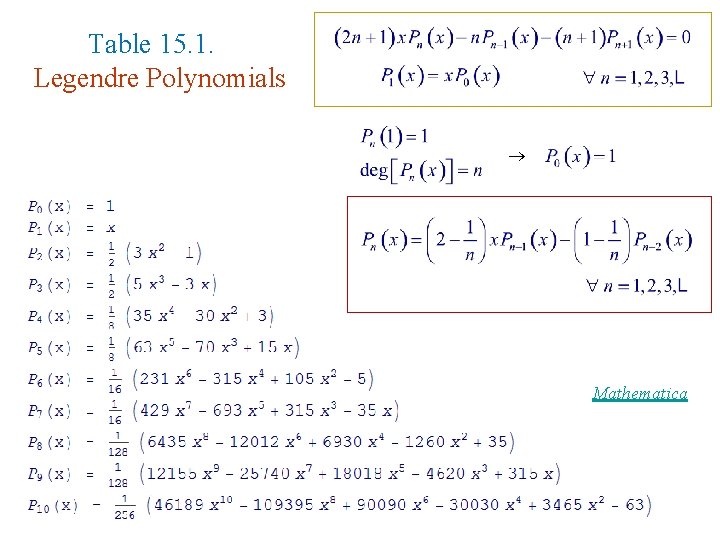
Computing coefficients is the process of measuring how much the original function overlaps with each basis element. Source: SlideToDoc
More complex functions are handled the same way. Even if a function does not terminate at a low degree the way x^2 does, summing from the lowest degree upward produces an approximation that converges toward the original function. How far to push the approximation degree N is a tradeoff between accuracy and cost.
Why Legendre Approximation Acts as an Inference Mechanism
Inference is the process of drawing conclusions that have not been computed directly from observed information. Legendre approximation summarizes a function with just a few coefficients rather than working with the entire function. Subsequent computation can then operate in coefficient space rather than on the original function.
For instance, suppose a system's state varies with input x, and f(x) is partially known from sensor data or simulation results. Computing the Legendre coefficients lets you answer questions like:
- What level are the values at overall?
- Does the value increase or decrease as input grows?
- Is the change linear or curved?
- Are the high-degree components large — i.e., does the function oscillate in a complex way?
- Is the low-degree representation sufficient, or is a more detailed model needed?
These questions can be answered without inspecting every point of the original function, because a handful of coefficients already captures the large-scale structure.
Legendre approximation therefore means more than simple curve fitting. It compresses the state of a function, supports judgment on that compressed representation, and refines the degree only when greater precision is needed.
The Parallel with Monte Carlo Tree Search
Monte Carlo Tree Search and Legendre approximation solve different problems. MCTS finds good paths in search problems with large branching factors. Legendre approximation expresses the shape of a continuous function or dataset with a small number of coefficients.
Both, however, avoid brute-forcing the full space. MCTS does not expand every possible path to completion; it concentrates computation on promising branches. Legendre approximation does not carry every fine detail of a function; it captures the important structure starting from the lowest-degree components.
In summary:
- Monte Carlo Tree Search: reduces a large search space via sampling and score updates.
- Legendre approximation: reduces a complex function space via orthogonal bases and coefficients.
- What they share: both produce a representation suitable for decision-making through approximate rather than exhaustive computation.
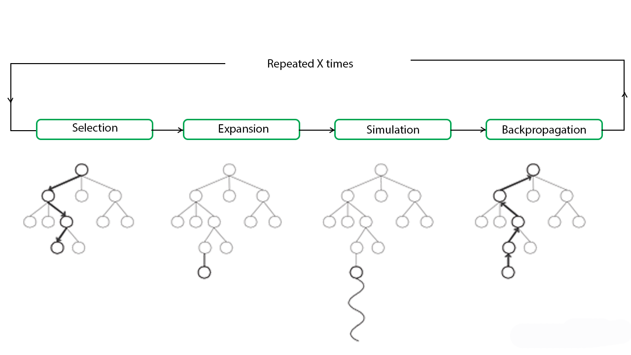
MCTS concentrates computation on promising paths rather than expanding the entire search space. Source: GeeksforGeeks
This perspective is also useful in structured reasoning systems like Graph RAG. When exhaustively exploring all paths in a graph is infeasible, you can allocate budget to promising paths the way MCTS does. Conversely, when a continuous scoring function, ranking function, response quality function, or cost function behaves in a complex way, you can summarize it in coefficient form the way Legendre approximation does.
One is approximation over path search; the other is approximation over function representation. Both recast the problem into a computationally tractable form, placing them in the same family of thinking.
Practical Applications
Legendre polynomials are a practical computational tool, not merely mathematical decoration. They appear most prominently in numerical analysis and physical computation — in spherical coordinate problems, partial differential equations, spectral methods, and numerical integration.
Gauss-Legendre quadrature uses the roots of Legendre polynomials to approximate integrals. Rather than evaluating the integrand at every point, it achieves high accuracy using a carefully chosen set of evaluation points and weights. This too embodies the core philosophy of approximate computation.
From a machine learning or inference system perspective, the approach can be understood as converting a function into a feature vector. When the input-output relationship of a model is available, storing it as Legendre coefficients rather than directly can then support comparison, compression, interpolation, and prediction downstream.
Concrete scenarios include:
- Approximating a model's performance curve as a function of a parameter
- Summarizing the shape of a cost or quality function over time
- Compressing simulation results into low-degree coefficients
- Representing an uncertain response scoring function in a polynomial basis
- Replacing a complex optimization objective with a tractable approximation
The important caveat is that Legendre approximation is not always the right answer. It is a strong choice when the function is well-behaved on [-1, 1], polynomial approximation is meaningful, and the low-degree structure is sufficiently strong.
Why the Input Interval Is Mapped to [-1, 1]
Legendre polynomials are defined on [-1, 1] by default. Real data, however, may have input ranges like 0 to 100, or a time axis from 0 to T. In these cases, a linear transformation maps the input to [-1, 1]:
x = 2(t - a) / (b - a) - 1
This makes x = -1 when t = a and x = 1 when t = b, mapping the original domain onto the standard interval where the polynomials are defined.
This transformation is small but essential. Without properly aligning the interval, orthogonality does not behave as expected. Legendre approximation is not just about using polynomials — it is about using polynomials that are mutually orthogonal on a specific interval.
![Diagram showing the transformation of input interval [a, b] to the Legendre standard interval [-1, 1]](/uploads/images/20260512_c568ed666d232db9.svg)
To apply Legendre approximation, the actual input interval is mapped to the standard interval [-1, 1].
Higher Degree Is Not Always the Answer
Increasing the approximation degree improves expressive power — but not unconditionally. When data contains noise, high-degree polynomials may fit the noise as well as the signal. Computation becomes more expensive, and oscillation near the endpoints of the interval can grow unexpectedly.
In practice, it is better to start from low degree. Begin with P_0, P_1, P_2 to capture the large-scale structure, and increase the degree incrementally if the error is too large. A useful diagnostic is to check whether the high-degree coefficients are small: if they are, adding higher-degree terms is unlikely to yield much additional information.
This pattern recurs throughout approximate computation. Rather than aiming for a perfect model from the start, begin with the simplest possible representation and add complexity only as needed.
The Algorithm in Summary
As a concrete procedure, Legendre approximation works as follows:
Input: function f(x), approximation degree N, interval [a, b]

1. Map the input interval [a, b] to [-1, 1].
2. Prepare Legendre polynomials P_0(x) through P_N(x).
3. Compute coefficient a_n for each degree n.
4. Use a_0 P_0(x) + ... + a_N P_N(x) as the approximation.
5. If the error is too large, increase N; otherwise stop.
The output of this procedure is both an approximating function and a compact representation of the original function. Storing the coefficient list [a_0, a_1, ..., a_N] instead of the original function is enough to support a wide range of downstream judgments.
In One Sentence
Legendre approximation is an approximate inference method that decomposes a complex function into non-overlapping polynomial components and retains only the significant coefficients, converting the function into a tractable form.
Where Monte Carlo Tree Search reduces computation to find good paths in a large search space, Legendre approximation reduces representation to find the important shape in a large function space. Both are an algorithmic way of thinking that reshapes a problem — one where exhaustive search or exhaustive representation is infeasible — into something small and powerful.