When a token is converted to an embedding vector, a sentence becomes a sequence of numeric vectors. That much was covered in part 2. But there is still one thing missing from that sequence of vectors: order.
나는 밥을 먹었다 and 밥이 나를 먹었다 share quite a few of the same tokens. From the embedding layer's perspective, each token ID is an address pointing to a row in a table, and the vector pulled from that row encodes the token's meaning and usage. The problem is that self-attention, in its basic form, compares the entire input all at once. If only token embeddings are provided, the model has no direct way to know which position each token occupied.
The transformer therefore adds a positional vector to each token vector. The original transformer in Attention Is All You Need does not learn these positional vectors — it precomputes them using sine and cosine functions. This approach is sinusoidal positional encoding.
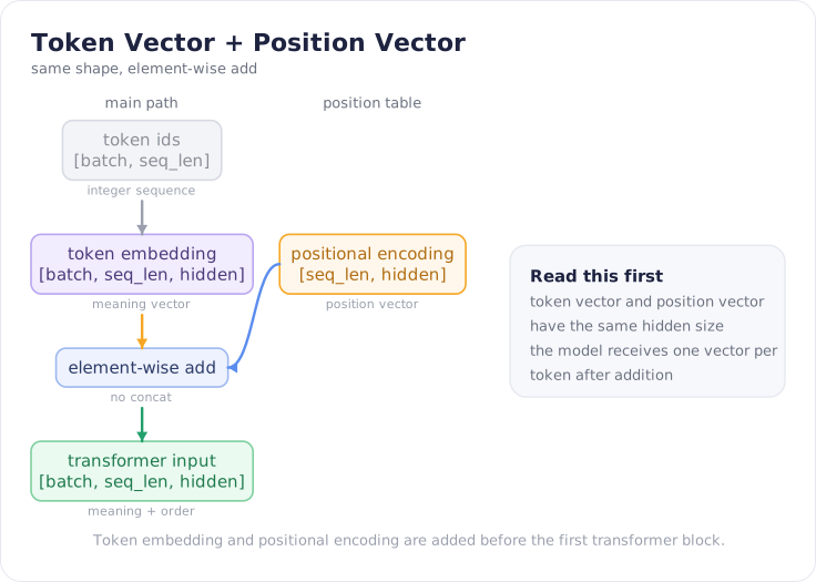
Figure 1. Token embeddings and positional encodings share the same hidden size and are combined via element-wise addition.
Why adding position to an embedding works
At first glance this seems odd. Token embeddings encode meaning; positional encodings encode position. Adding two pieces of information with different characters together sounds wrong. But that is exactly what happens.
The transformer's input vector is typically constructed like this:
x = token_embedding[token_ids] + positional_encoding[:seq_len]
In terms of shapes, it is even simpler:
token_ids              [batch, seq_len]
token_embedding        [batch, seq_len, hidden_size]
positional_encoding    [       seq_len, hidden_size]
input_to_transformer   [batch, seq_len, hidden_size]
If hidden_size is 768, then the token embedding is 768-dimensional and the positional encoding is also 768-dimensional. Adding two vectors of the same dimension yields a vector of the same dimension. From the model's perspective, the input vector is a mixture of token information and positional information.
This works because the layers that follow can decompose and recombine this mixed representation. The query, key, and value projections in self-attention multiply the input vector by learned weight matrices. Some heads will respond strongly to token semantics; others will be sensitive to positional differences. These orientations emerge during training — nobody has to manually declare that the first 384 dimensions carry meaning while the last 384 carry position.
There is also a practical engineering advantage to addition. The input shape stays the same regardless of sequence length. Concatenating token embeddings with positional encodings would increase the hidden size, forcing changes to every downstream projection matrix. Addition keeps the model architecture clean. It is a simple choice, but a powerful one.
Reading the sinusoidal positional encoding formula
The formula from the original paper is:
PE(pos, 2i)     = sin(pos / 10000^(2i / d_model))
PE(pos, 2i + 1) = cos(pos / 10000^(2i / d_model))
There are a lot of symbols, but each one is straightforward.
pos is the token's position — 0 for the first token, 1 for the second, and so on. Some implementations start from 1, but the principle is the same. i refers to the index of a pair of hidden dimensions. d_model is the hidden size — the same value typically called hidden_size in GPT-style models.
Even-indexed dimensions use sin; odd-indexed dimensions use cos. Dimensions 0 and 1 share the same frequency, one with sin and one with cos. Dimensions 2 and 3 use a slightly slower frequency. The wavelength grows longer as you move to higher dimensions.
Each position's positional encoding is therefore a vector obtained by slicing across multiple frequency waves at that position.
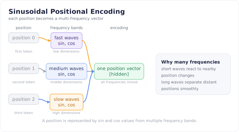
Figure 2. Each position holds sin and cos values from multiple frequencies, spread across the hidden dimension.
For a hidden size of 8, each position would look something like this. Real models use much larger dimensions — 512, 768, 4096, and beyond.
position 0 -> [sin(0/a0), cos(0/a0), sin(0/a1), cos(0/a1), ...]
position 1 -> [sin(1/a0), cos(1/a0), sin(1/a1), cos(1/a1), ...]
position 2 -> [sin(2/a0), cos(2/a0), sin(2/a1), cos(2/a1), ...]
The values at position 0 are not all zero. The sin terms are zero, but the cos terms are 1. This means the first position still gets a unique, non-trivial vector.
Dimensions with short wavelengths are sensitive to small positional changes — even a shift of 1 in position produces a noticeably different value. Dimensions with long wavelengths smoothly distinguish positions that are far apart. By mixing multiple frequencies, a single vector captures both fine-grained and coarse-grained positional structure.
Why sine and cosine specifically
Sine and cosine are continuous and periodic. A small change in position produces a small change in the positional vector. Position 10 and position 11 do not look like completely unrelated IDs — they carry a trace of being nearby. That property is well-suited for handling order.
Another advantage is that these functions make relative positions easy to handle linearly. Sine and cosine satisfy:
sin(a + b) = sin(a)cos(b) + cos(a)sin(b)
cos(a + b) = cos(a)cos(b) - sin(a)sin(b)
This means the encoding for position pos + k can be expressed as a linear combination of the sin and cos values at position pos and the sin and cos values of offset k. The internal operations of a transformer are mostly linear transformations combined with attention. The sinusoidal encoding provides a structure that makes it easy for those operations to pick up on relative distance patterns.
Absolute position is rarely what matters most in language. What comes up far more often is relative position: does 는 immediately follow 나? Is the verb near the end of the sentence? How many tokens after an opening parenthesis does the closing one appear? Sinusoidal positional encoding gives the model a coordinate system that makes learning these kinds of relative position rules straightforward.
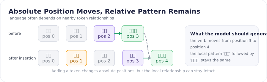
Figure 3. Inserting a token at the start of a sentence shifts all absolute positions, but the relative relationships between neighboring tokens stay intact.
In 나는 오늘 밥을 먹었다, 먹었다 might sit at position 4. In 나는 정말 오늘 밥을 먹었다, it shifts to position 5. The absolute position changed, but the structure — verb following 밥을 — is preserved. That is the kind of pattern a language model needs to generalize over.
Comparison with learned position embeddings
Positional encoding does not have to use sine and cosine. BERT-style models widely adopted the approach of learning a position embedding table. Like the token embedding table, it has a row for each position (0, 1, 2, …) and training updates those values.
Learned position embeddings are simple and perform well. The model directly adjusts position vectors to match the positional patterns it sees in data. For encoder models with a fixed maximum sequence length, this is a natural fit — BERT, for example, caps input length at 512 tokens.
The sinusoidal approach has no learnable parameters. Given a maximum length, the table can be precomputed, and in principle it can generate values for positions longer than anything seen during training. That sounds appealing, but it does not automatically solve long-context generalization. The attention layers, the length distribution of training data, normalization, and post-training alignment all play a role. Just extending the positional encoding does not turn a 2K-context model into a 128K-context model.
This is the point where beginners most often get confused. Sinusoidal positional encoding is a method for computing a position vector at any index. The ability to handle long contexts properly requires the entire model to be trained and aligned on long-context data. Being able to produce a position vector is not the same as reasoning well over long contexts.
A small PyTorch implementation
Sinusoidal positional encoding is short to implement. The code below produces a [max_len, d_model] matrix.
import math
import torch


def sinusoidal_positional_encoding(max_len: int, d_model: int) -> torch.Tensor:
    pe = torch.zeros(max_len, d_model)

    position = torch.arange(0, max_len, dtype=torch.float32).unsqueeze(1)
    div_term = torch.exp(
        torch.arange(0, d_model, 2, dtype=torch.float32)
        * (-math.log(10000.0) / d_model)
    )

    pe[:, 0::2] = torch.sin(position * div_term)
    pe[:, 1::2] = torch.cos(position * div_term)
    return pe


pe = sinusoidal_positional_encoding(max_len=8, d_model=6)
print(pe.round(decimals=4))
The output looks roughly like this:
tensor([[ 0.0000,  1.0000,  0.0000,  1.0000,  0.0000,  1.0000],
        [ 0.8415,  0.5403,  0.0464,  0.9989,  0.0022,  1.0000],
        [ 0.9093, -0.4161,  0.0927,  0.9957,  0.0043,  1.0000],
        [ 0.1411, -0.9900,  0.1388,  0.9903,  0.0065,  1.0000],
        [-0.7568, -0.6536,  0.1846,  0.9828,  0.0086,  1.0000],
        [-0.9589,  0.2837,  0.2300,  0.9732,  0.0108,  0.9999],
        [-0.2794,  0.9602,  0.2749,  0.9615,  0.0129,  0.9999],
        [ 0.6570,  0.7539,  0.3192,  0.9477,  0.0151,  0.9999]])
Dimensions 0 and 1 oscillate rapidly. Dimensions 4 and 5 barely change across the max_len=8 range. As d_model grows and sequences get longer, the slow-wavelength dimensions take on the job of distinguishing distant positions.
When feeding this into an actual transformer block, broadcast over the batch dimension as follows:
batch_size = 2
seq_len = 8
d_model = 6

token_embeddings = torch.randn(batch_size, seq_len, d_model)
pe = sinusoidal_positional_encoding(max_len=seq_len, d_model=d_model)

x = token_embeddings + pe.unsqueeze(0)
print(x.shape)  # torch.Size([2, 8, 6])
The positional encoding here receives no gradient updates. With a learned position embedding, you would create nn.Embedding(max_len, d_model) and let the optimizer update those weights alongside everything else.
How positional information is used inside attention
Self-attention derives query, key, and value from each token:
q_i = x_i W_Q
k_j = x_j W_K
score(i, j) = q_i · k_j
Here x_i is the token embedding with positional encoding already added in. Attention scores are therefore influenced by both token semantics and position. When computing how much token i attends to token j, both their content and their positions factor into the score.
For example, a head might learn to attend strongly to the immediately preceding token, while another might focus near the beginning of the sentence or around separator tokens. Attention map visualizations frequently show heads that track along the diagonal — these are heads dealing with adjacent-token relationships.
This should not be overstated. Having positional encoding in the input does not mean the model automatically understands grammar. It simply means the model gets better raw material to work with than it would have without positional information. Everything else emerges from large-scale next-token prediction training.
Modern Models Prefer RoPE
The original transformer's sinusoidal positional encoding is still an elegant design. That said, modern decoder-only LLMs more commonly use RoPE instead of adding a position vector to the input embedding. RoPE rotates the query and key vectors according to position, which injects relative position information more directly into the attention scores.
Anyone who has worked with Qwen or Llama-family models will have run into RoPE-related config fields: rope_theta, rope_scaling, context extension settings, and so on. This is also where you see why positional encoding becomes a problem when extending context length. A model isn't simply a machine that accepts more tokens — it has attention patterns learned under a specific length and position distribution.
That said, sinusoidal positional encoding is still the right place to start. It makes the core idea — injecting order information into token embeddings — as clear as it gets. RoPE, ALiBi, and learned absolute position embeddings are all variations that implement this same idea in different ways.
Why This Belongs Between Part 2 and Part 3
The embedding layer maps token IDs to vectors. Positional encoding gives those vectors an ordering coordinate. Only after both are combined does the transformer block receive the input it needs to process a sequence.
The tokenizer splits a sentence into token IDs, the embedding layer maps those IDs to dense vectors, and positional encoding stamps a position into each vector. The self-attention mechanism we'll look at next takes this input and computes relationships across every pair of tokens. This is where the transformer starts to look like a transformer.