In Part 1, the tokenizer converted a sentence into an array of token IDs. For example, the sentence "나는 밥을 먹었다" becomes a numeric array like [8172, 392, 10491, 1837]. At this point, the text is gone — only integers remain.
The transformer doesn't read these integers as-is. The number 8172 carries no meaning on its own. A larger ID doesn't mean a stronger word, and a nearby ID doesn't mean a similar word. A token ID is essentially an address — an index into the vocabulary table.
The layer that converts these addresses into vectors the model can compute with is the embedding layer.
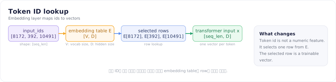
Each token ID points to a row in the embedding table, and the result of that row lookup becomes the transformer's input vector.
Token IDs are meaningless integers
Let's revisit what the tokenizer produces.
입력 문장: 나는 밥을 먹었다
토큰:      ["나는", " 밥", "을", " 먹었다"]
토큰 ID:   [8172, 392, 10491, 1837]
A human reading "나는", "밥", and "먹었다" immediately senses sentence structure. From the model's perspective, four integers arrive. Feeding these integers directly into attention causes problems: the numerical ordering of IDs gets treated as if it reflects semantic relationships.
10491 is about 26 times larger than 392. But there's no interpretation in which "을" carries 26 times more meaning than "밥". Token IDs are not sortable numeric features — they're just lookup keys.
So the first step converts IDs into vectors.
8172  ->  [ 0.12, -0.03,  0.77, ...,  0.08]
392   ->  [-0.41,  0.56,  0.02, ..., -0.19]
10491 ->  [ 0.09,  0.11, -0.64, ...,  0.33]
1837  ->  [ 0.48, -0.22,  0.17, ...,  0.05]
The length of each vector is determined by the model. In GPT-family models, this is typically called hidden_size, d_model, or n_embd. For a model with d_model=4096, a single token is represented by 4096 floating-point numbers. With a sequence of 128 tokens, the tensor shape after the embedding layer is roughly [128, 4096]. Including a batch dimension, it becomes [batch_size, sequence_length, hidden_size].
The embedding layer is a giant lookup table
The structure of an embedding layer is straightforward.
embedding table shape = [vocab_size, hidden_size]
With a vocabulary of 50,000 and a hidden size of 768, the embedding table has 50,000 × 768 parameters. When token ID 8172 comes in, the model retrieves row 8172. That's it. It may look like a matrix multiplication, but from an implementation standpoint it's just a row lookup.
Here's a minimal example:
import torch
import torch.nn as nn

embedding = nn.Embedding(num_embeddings=5, embedding_dim=3)

input_ids = torch.tensor([0, 2, 4])
x = embedding(input_ids)

print(x.shape)
# torch.Size([3, 3])
num_embeddings is the vocabulary size. embedding_dim is the number of dimensions used to represent each token. Passing [0, 2, 4] as input_ids retrieves rows 0, 2, and 4 from the embedding table.
The math is even shorter:
E: embedding table, shape [V, D]
input_ids = [t0, t1, t2, ...]
output[i] = E[input_ids[i]]
Here V is vocabulary size and D is hidden size. The embedding layer itself has no access to context. The same token ID always starts from the same initial vector. The embedding layer alone can't determine whether "배" means fruit, a body part, or a ship. That disambiguation happens as subsequent self-attention and feed-forward layers mix in information from surrounding tokens.
This distinction matters. An embedding vector is a token's base coordinate; the hidden state after passing through transformer blocks is a context-aware coordinate.
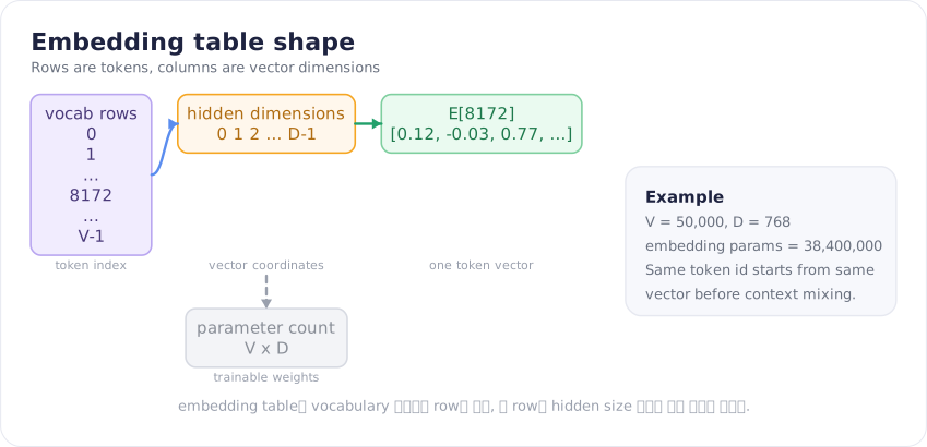
The embedding table has as many rows as the vocabulary size, and each row is a learnable vector of length hidden_size.
How vectors acquire meaning
A freshly initialized embedding table is essentially random. Before training, there is no linguistic relationship between row 8172 and row 392. As the model trains on next-token prediction, these coordinates are continuously adjusted.
Tokens that frequently appear in similar positions within sentences — and that are useful for predicting similar next tokens — tend to move in similar directions during training. "강아지" (dog) and "고양이" (cat) are different tokens, but both commonly appear in contexts involving animals, as subjects, as objects, and as things being described. As a result, they end up relatively close to each other in embedding space. This intuition became well-known during the Word2Vec era, and the same underlying principle applies to input embeddings in transformers.
That said, interpreting LLM embeddings as a word dictionary quickly hits limits. Modern tokenizers don't split text purely on word boundaries. "unbelievable" might be split into un, believ, able; in Korean, particles and verb endings may become separate tokens, or text may be split into byte-level pieces. Each row in the embedding table represents one token's coordinate — not a complete word.
Even so, the model combines these fragments to construct meaning. Even when "먹", "었", "다" arrive separately, they get folded into a contextual representation of a past-tense predicate as they pass through multiple layers. The more aggressively a tokenizer fragments a language, the more work goes into that recombination. A longer tokenized sequence means more tokens for attention to process and more embedding lookups to perform. This is why tokenizer quality is not something to overlook when building Korean-language models.
Parameter count of the embedding layer
The embedding layer is larger than it might seem. Even in smaller BERT-family models, the input embedding alone can consume tens of millions of parameters once vocabulary and hidden size grow.
vocab_size = 50,000
hidden_size = 4,096

embedding parameters = 50,000 x 4,096
                     = 204,800,000
In FP16, each parameter takes 2 bytes, so the token embedding table alone occupies about 390 MiB. Factor in output projections, optimizer states, and gradients during training, and the memory footprint grows considerably.
These numbers illustrate that tokenizer design and model size are directly coupled. A larger vocabulary lets you represent sentences with fewer tokens, but the embedding table grows. A smaller vocabulary shrinks the embedding table but makes sentences longer. Neither side is free.
This trade-off comes up regularly in practice. Models handling Korean, Japanese, code, mathematical notation, or domain-specific strings feel the impact of vocabulary design directly in cost. More tokens consume the context window faster and increase attention computation. Conversely, inflating the vocabulary makes it harder to train good embeddings for rare tokens.
Input embedding and output embedding
A language model converts input tokens to embeddings, passes them through multiple transformer blocks, and ultimately needs to produce a probability distribution over the next token. That final step requires a projection that maps the hidden state to a logit vector of size equal to the vocabulary.
hidden state shape = [sequence_length, hidden_size]
output logits shape = [sequence_length, vocab_size]
If the hidden state at the last position is [4096], the model maps it to [vocab_size] scores, one per token candidate. Applying softmax yields the next-token probability distribution.
A common design choice here is to share the input embedding table with the output projection weights — a technique called weight tying. Press and Wolf showed that tying input and output embeddings can reduce parameter count while also improving language model performance.
Structurally, it looks like this:
input:  token id -> embedding table row -> hidden vector
output: hidden vector -> vocab logits computed with the same weights as the embedding table
This makes intuitive sense: the coordinate system used to interpret incoming tokens is aligned with the coordinate system used to score outgoing token candidates. Not every model does this, but it's a common design in decoder-only LLMs.
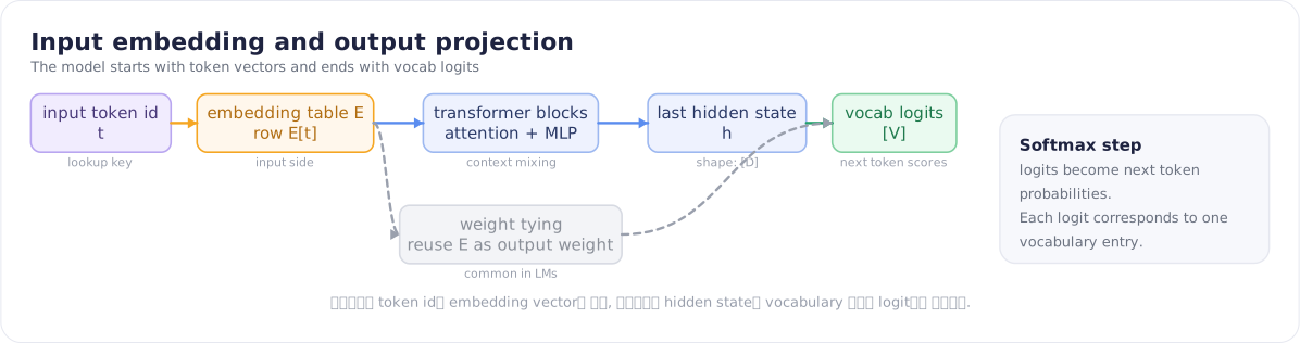
On the input side, a token ID becomes an embedding vector. On the output side, the hidden state is projected onto logits across the entire vocabulary.
Embedding here shares its name with embedding in semantic search
In practice, the word "embedding" refers to two different things.
One is the token embedding covered here: the parameters in the model's first layer that convert token IDs into hidden vectors. These are learned parameters and are part of the model architecture.
The other is the sentence or document embedding used in RAG and semantic search. Here, an entire sentence or document is compressed into a single vector for retrieval purposes — for example, finding documents similar to the query "환불 정책" in a vector database.
Both are vector representations, so they're related. But their roles differ. Token embeddings are the starting point for internal model computation; sentence embeddings are an output artifact used for external search or clustering. The shared name causes frequent confusion when first learning the field.
A quick comparison:
| token embedding | sentence/document embedding | |
|---|---|---|
| Input | Token ID | Sentence, document, chunk |
| Output | Per-token vector | Single vector for the text unit |
| Location | Internal LLM layer | Output of an embedding model |
| Primary use | Transformer input representation | Search, similarity, clustering |
| Context awareness | Weak at the embedding layer alone | Typically reflects full context |
A single embedding vector carries no positional information
After passing through the embedding layer, each token becomes a vector. The problem is that these vectors alone contain no information about where a token appears in the sequence.
[나는] [밥을] [먹었다]
[먹었다] [밥을] [나는]
These two sequences have similar token compositions but different meanings. Self-attention computes relationships between tokens, but if the input vectors carry no position information, the model has no signal for "which position is this token at?" Transformers solve this by adding position information to the token embeddings.
Attention Is All You Need used sinusoidal positional encoding: fixed vectors built from sin and cos patterns are generated for each position and added to the token embeddings.
x = token_embedding + positional_encoding
This one line lets the model treat "나는" at position 0 differently from "나는" at position 5, even though they have the same token ID. Modern LLMs commonly use RoPE instead of absolute sinusoidal encoding, but the starting point is the same: mix the token's semantic coordinate with a positional coordinate to form a proper sequence representation.
Sinusoidal positional encoding deserves its own treatment in Part 2.5. The formula is short, but explaining why sin and cos are used, and how positional differences propagate into attention, would derail the flow of this post.
The embedding layer keeps moving during training
Any discussion of fine-tuning that glosses over the embedding layer is incomplete. Training on new domain data doesn't only change the transformer blocks. Depending on the training configuration, token embeddings update too. Tokens that appear repeatedly in specific patterns — domain-specific terminology, code snippets, medical terms, legal vocabulary — will have their coordinates shifted to fit the surrounding distribution.
This shift can be beneficial. It can make the model follow particular output formats more reliably, or handle frequently used term combinations more stably. It can also degrade general language modeling. Because the embedding layer is the entry point for the entire network, large coordinate shifts here change the input distribution that downstream layers were calibrated to expect.
This is why full fine-tuning on small datasets requires care. The model doesn't store new knowledge like a database entry. It re-calibrates the probability distribution across tokens. The embedding layer is part of that distribution. Earlier posts described domain fine-tuning failures in terms of corrupting the next-token distribution — and the embedding layer is the furthest-upstream point where that corruption can begin.
Tracking shapes directly cuts through the confusion
Below is the shape of the data right before it enters a decoder-only transformer. Variable names differ across models, but the flow is nearly identical.
import torch
import torch.nn as nn

batch_size = 2
seq_len = 4
vocab_size = 50000
hidden_size = 768

input_ids = torch.randint(0, vocab_size, (batch_size, seq_len))
# shape: [2, 4]

tok_embedding = nn.Embedding(vocab_size, hidden_size)

x = tok_embedding(input_ids)
# shape: [2, 4, 768]
x[:, 0, :] is the first token vector for each item in the batch. x[0, :, :] is all token vectors for the first sequence. x[0, 2, :] is the single 768-dimensional vector representing the third token in the first sequence.
If you're also using learned position embeddings, you add them like this:
max_seq_len = 1024
pos_embedding = nn.Embedding(max_seq_len, hidden_size)

positions = torch.arange(seq_len).unsqueeze(0)
# shape: [1, 4]

x = tok_embedding(input_ids) + pos_embedding(positions)
# shape: [2, 4, 768]
Broadcasting lets the [1, 4, 768] position vectors be added across the entire batch. Every sequence in the batch receives the same position embedding for the same position. Even the same token gets a different final input vector if it appears at a different position.
The sinusoidal approach doesn't learn a position table via nn.Embedding — it computes position vectors analytically from a formula. Learned position embeddings are trainable parameters; sinusoidal positional encodings are a fixed function. That difference becomes immediately clear when you print the values side by side, which is what the next post will do.
Putting parts 1 and 2 together
The tokenizer converts a string into token IDs from the model's vocabulary. The embedding layer converts those IDs into dense vectors the model can compute over. Position information is then added, and the transformer blocks use attention to mix context across the sequence.
text
-> tokenizer
-> input_ids
-> token embedding
-> position 정보 추가
-> transformer blocks
-> logits
-> next token probabilities
Understanding this pipeline makes LLMs a lot less mysterious. Text doesn't magically become intelligence — strings become IDs, IDs become vectors, and vectors pass through layers until they become a probability distribution over the next token.
Part 2.5 will break down sinusoidal positional encoding through both the math and the code. The plan is to work through why a formula like pos / 10000^(2i/d_model) appears, and how alternating sin and cos encodes relative position differences — with actual numbers printed out at each step.